
Rectilinear Kinematics
Finding Velocity & Position from a Time-Dependent Acceleration
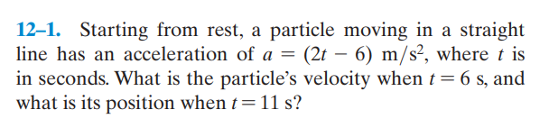
A particle begins its motion from rest along a straight-line path. Its acceleration varies with time according to
\( a = (2t – 6) \;\text{m/s}^2 \), where \( t \) is measured in seconds.
Determine the velocity of the particle at \( t = 6\;\text{s} \), and find its displacement from the starting point when \( t = 11\;\text{s} \).
What We Know
- Initial velocity: \( v_0 = 0 \;\text{m/s} \) (starts from rest)
- Initial position: \( s_0 = 0 \;\text{m} \) (origin taken as start point)
- Acceleration law: \( a(t) = (2t – 6) \;\text{m/s}^2 \)
- Find velocity at \( t = 6\;\text{s} \)
- Find position at \( t = 11\;\text{s} \)
Why direct integration? — The acceleration here is an explicit function of time, not a constant. Kinematic equations like \( v = v_0 + at \) only work for constant acceleration. Since \( a(t) \) changes every instant, we must integrate \( a \) to get \( v \), then integrate \( v \) to get \( s \). This is the fundamental approach for variable acceleration problems.
Step 1
Relate Acceleration to Velocity via Differentiation Definition
By definition, acceleration is the time-rate of change of velocity:
\[ a = \frac{dv}{dt} \]
Rearranging, we separate variables — velocity on the left, time on the right — to prepare for integration:
\[ dv = a \; dt = (2t – 6)\; dt \]
Physical meaning: Each infinitesimal \( dv \) (tiny change in speed) is produced by the acceleration acting over a tiny time slice \( dt \). Summing all of these — integrating — gives the total velocity change over any time interval.
Step 2
Integrate to Obtain the Velocity Expression
Apply definite integration from the known initial state \((v = 0 \text{ at } t = 0)\) up to a general time \( t \):
\[
\int_0^{v} dv = \int_0^{t} (2t – 6)\; dt
\]
Evaluating both sides:
\[
v \;\Big|_0^{v} = \left[ t^2 – 6t \right]_0^{t}
\]
\[ \boxed{v(t) = t^2 – 6t} \quad \text{(m/s)} \tag{1} \]
Note on sign: For \( 0 < t < 6\;\text{s} \), the term \( (2t-6) \) is negative, meaning the particle is actually decelerating initially (it starts at rest and the acceleration acts to pull it backward before \( t = 3\;\text{s} \) when \( a = 0 \)). After \( t = 6\;\text{s} \), \( a \) is positive and the particle accelerates forward again.
Step 3
Evaluate Velocity at \( t = 6\;\text{s} \)
Substitute \( t = 6 \) into equation (1):
\[
v(6) = (6)^2 – 6(6) = 36 – 36
\]
\( v \big|_{t=6\,\text{s}} = 0 \;\text{m/s} \)
Why zero? The particle started from rest, decelerated, momentarily stopped (at \( t = 3\;\text{s} \), it hits its most negative velocity of \(-9\;\text{m/s}\)), then the positive acceleration brought it back to exactly zero speed again at \( t = 6\;\text{s} \). It has returned to the same speed — though not the same position — as at the start.
Step 4
Relate Velocity to Position
Velocity is the time-rate of change of position \( s \):
\[ v = \frac{ds}{dt} \implies ds = v\; dt \]
Substituting the velocity expression from equation (1):
\[ ds = \left(t^2 – 6t\right) dt \]
Step 5
Integrate to Obtain Position and Evaluate at \( t = 11\;\text{s} \)
Integrate from the known initial position \( s = 0 \) at \( t = 0 \):
\[
\int_0^{s} ds = \int_0^{t} \left(t^2 – 6t\right) dt
\]
\[
s \;\Big|_0^{s} = \left[ \frac{t^3}{3} – 3t^2 \right]_0^{t}
\]
\[ \boxed{s(t) = \frac{t^3}{3} – 3t^2} \quad \text{(m)} \tag{2} \]
Now substitute \( t = 11\;\text{s} \):
\[
s(11) = \frac{(11)^3}{3} – 3(11)^2 = \frac{1331}{3} – 363
\]
\[
s(11) = 443.67 – 363
\]
\( s \big|_{t=11\,\text{s}} \approx 80.67 \;\text{m} \)
Interpreting the result: The positive value confirms that at \( t = 11\;\text{s} \), the particle is 80.67 m ahead of (in the positive direction from) where it started. Even though the particle moved backward during \( 0 < t < 6\;\text{s} \) (since \( v < 0 \) in that window), the strong forward motion after \( t = 6\;\text{s} \) more than compensates. The net displacement is positive.
✦ Final Answers
Velocity at \( t = 6\;\text{s} \): \( v = 0 \;\text{m/s} \)
Position at \( t = 11\;\text{s} \): \( s \approx 80.67 \;\text{m} \)