Modeling and simulation of mechanical systems

Report
Question

Please briefly explain why you feel this question should be reported.

Report
Cancel

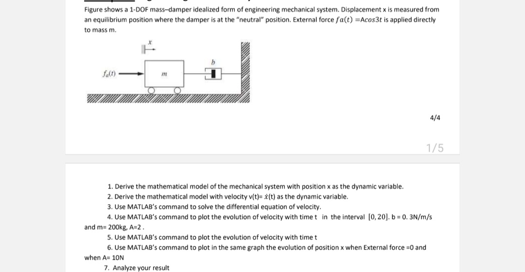
Figure shows a 1-DOF mass-damper idealized form of engineering mechanical system. Displacement x is measured from an equilibrium position where the damper is at the “neutral” position. External force fa(t) =Acos3t is applied directly to mass m.

1. Derive the mathematical model of the mechanical system with position x as the dynamic variable.

2. Derive the mathematical model with velocity v(t)= x(t) as the dynamic variable.

3. Use MATLAB’s command to solve the differential equation of velocity.

4. Use MATLAB’s command to plot the evolution of velocity with time t in the interval [0, 20]. b = 0. 3N/m/s and m= 200kg, A=2.

5. Use MATLAB’s command to plot the evolution of velocity with time t

6. Use MATLAB’s command to plot in the same graph the evolution of position x when External force =0 and

when A= 10N

7. Analyze your result

MathJax Example

Answer ( 1 )

  1. Please briefly explain why you feel this answer should be reported.

    Report
    Cancel
    % Parameters
    b = 0.3; % N/m/s
    m = 200; % kg
    A_values = [0, 10]; % N
    tspan = [0 20]; % Time interval

    % Initial conditions (assuming v(0) = 0)
    v0 = 0;

    % Define the system of equations for velocity
    ode_velocity = @(t, v, A) (A – b*v) / m;

    % Solve and plot for each A value
    figure;
    hold on;
    for A = A_values
    [t, v] = ode45(@(t, v) ode_velocity(t, v, A), tspan, v0);
    plot(t, v, ‘DisplayName’, [‘A = ‘ num2str(A) ‘ N’]);
    end
    hold off;

    % Plot settings for velocity
    xlabel(‘Time (s)’);
    ylabel(‘Velocity v(t) (m/s)’);
    title(‘Evolution of Velocity for Different External Forces’);
    legend show;
    grid on;

    % Solve for position x(t) by integrating velocity
    figure;
    hold on;
    for A = A_values
    [t, v] = ode45(@(t, v) ode_velocity(t, v, A), tspan, v0);
    x = cumtrapz(t, v); % Integrate velocity to get position
    plot(t, x, ‘DisplayName’, [‘A = ‘ num2str(A) ‘ N’]);
    end
    hold off;

    % Plot settings for position
    xlabel(‘Time (s)’);
    ylabel(‘Position x(t) (m)’);
    title(‘Evolution of Position for Different External Forces’);
    legend show;
    grid on;

Leave an answer

Browse

By answering, you agree to the Terms of Service and Privacy Policy.