Share
Consider a Shallow neural network with the following parameters. ϕ = {ϕ0, ϕ1, ϕ2, ϕ3, θ10, θ11, θ20, θ21, θ30, θ31} = {−0.23,−1.3, 1.3, 0.66,−0.2, 0.4,−0.9, 0.9, 1.1,−0.7}. Assuming the following activation functions, draw the input-output relationship highlighting the linear regions.
ReportQuestion
Please briefly explain why you feel this question should be reported.
Consider a Shallow neural network with the following parameters.
ϕ = {ϕ0, ϕ1, ϕ2, ϕ3, θ10, θ11, θ20, θ21, θ30, θ31} = {−0.23,−1.3, 1.3, 0.66,−0.2, 0.4,−0.9, 0.9, 1.1,−0.7}.
Assuming the following activation functions, draw the input-output relationship highlighting the linear regions.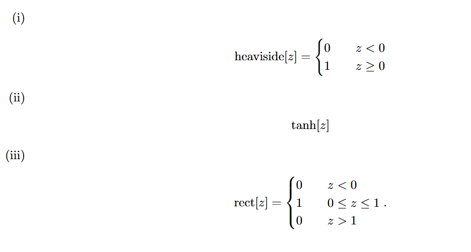
Answers ( 3 )
Please briefly explain why you feel this answer should be reported.
Please briefly explain why you feel this answer should be reported.
Please briefly explain why you feel this answer should be reported.